Run-length encoding in OMF object files

The Relocatable Object Module Format (OMF) is a file format designed by Intel for their 80×86 processors. It was a commonly used output format of 16-bit DOS compilers and assemblers usually with the extension .OBJ.

The file format consists of a series of records. Here we will concentrate on the Logical Iterated Data Record (LIDATA) which has an interesting method of run-length encoding data. The record consists of a data block. A data block contains a repeat count, a block count, and data. The repeat count specifies how many times the data in the data block should be repeated. The data can consist of either a number of more data blocks as specified by block count, or if block count is zero, a series of up to 255 data bytes. We can illustrate this recursive scheme with data blocks nested within another data block as a box which can contain either more boxes or some text. The repeat count of each box is shown in the upper left corner of the box.

A box can contain more boxes or a string

In this example we have a box which contains two more boxes, and the second of these does itself contain two more boxes. We can label the boxes in the following way. The outermost box we call b1, the two boxes inside b1 we call b1.1 and b1.2. The box b1.2 contains two more boxes which we call b1.2.1 and b1.2.2. Now, to see what final string this scheme will produce we process the boxes from left to right and concatenate the strings together. The box b1.1 will produce the string “ABC” repeated 1 time so the string of b1.1 is “ABC”. The next box, b1.2 contains two boxes, b1.2.1 which produces the string “DEF” and b1.2.2 which produces “GHGH”. Putting these together and then repeating twice we get that b1.2 produces the string “DEFGHGHDEFGHGH”. Putting b1.1 and b1.2 together we get the string “ABCDEFGHGHDEFGHGH”. The box b1 contains a repeat count of two so the final string will be “ABCDEFGHGHDEFGHGHABCDEFGHGHDEFGHGH”. We can express this more simply using algebra on strings like in the Python language as 2*(1 * “ABC” + 2*(1 * “DEF” + 2 * “GH”)).

The actual data block in the file has the following format:

Data Block

Repeat Count is a 16-bit value and determines how many times the Data field is repeated.

Block Count is a 16-bit value which determines how the Data field is interpreted. A value of 0 indicates that the Data field contains a 1-byte count value followed by count data bytes. The data bytes will be repeated as many times as specified by the repeat count. If the block count field is not zero it indicates that the data field is composed of one or more data blocks, as many as indicated by the block count value. The data blocks considered as one unit is repeated as specified by the repeat count.

This format can be a very compact way of representing repetitive data. For example consider the string 300*(100 * “ABC” + 100*(20 * “DEF” + 30 * “GHI”)) in Python notation. Illustrated with boxes it would look like this:

Large string

The length of this string is about 4.6 million bytes. As a data block in an LIDATA record this would take up 4 bytes for each of the five data blocks and 4 bytes for each of the 3 strings which gives a total of 4*5 + 4*3 = 32 bytes! Quite the saving. As a comparison, zip compresses this string to 36k, 7-zip does a lot better with 3.5k.

Sidenote: Assemblers like MASM and TASM include a DUP command which can save you a lot of typing. To declare an array of 100 bytes with the value 1 you can write DB 100 DUP(1). I haven’t investigated if the DUP command can be nested or if when using it the assembler will make use of the LIDATA nested block structure. If so, was the DUP command introduced to take advantage of the LIDATA record or was the LIDATA record created based on the DUP command? If someone knows the history, please leave a comment!

Sometimes seeing is not believing

In a lecture at MIT by Professor Walter Lewin which can be seen at 8.02x – Lect 16 – Electromagnetic Induction, Faraday’s Law, Lenz Law, SUPER DEMO he demonstrates an interesting experiment whereby he connects two voltmeters on opposite sides of a loop containing two resistors of 1 Ohm and 9 Ohm. Inside the loop he generates an increasing magnetic field which produces an EMF of 1 Volt in the loop. The voltmeter on the right of the 9 Ohm resistor reads .9 Volt and the one on the left of the 1 Ohm resistor reads -.1 Volt. At first glance this seems like a paradox, the voltmeters are connected to the same two points and should therefor show the same value!

Lewin experiment

In the middle loop there is a varying magnetic field which increases in the direction towards you and at a moment in time it produces an EMF of 1V.

EMF induced

Using Faraday’s law of induction:

$$\oint \mathbf{E}\cdot \mathrm{d}\mathbf{l} = -\frac{\mathrm{d}\Phi}{\mathrm{d}t}$$

and Ohm’s law we can easily calculate the current in the loop. We assume a current going counterclockwise and go around the loop in the direction of the current. \(R_{\mathrm{left}}\cdot I+R_{\mathrm{right}}\cdot I = -\frac{\mathrm{d}\Phi}{\mathrm{d}t}\) or \(1\cdot I+9\cdot I = -1\) which gives \(I=-0.1\mathrm{A}\). So the actual direction of the current will be clockwise which also follows from Lenz’s law.

Induced current

We can model the voltmeters as very large resistors and analyse the currents produced in the left and and the right one respectively. The magnetic field is so small outside of the middle loop that the EMF induced in the voltmeters can be neglected.

Currents through the voltmeters

Using KVL and Ohm’s law in the left loop: $$ 10^7i_1 + (i_1+I) = 0 $$

And doing the same for the right loop: $$ 10^7i_2+9(i_2-I) = 0 $$

And finally we use Faraday’s law for the middle loop:

$$ 9(I-i_2)+(I+i_1)=1 $$

Solving these equations we get:

$$ \begin{align*} i_1 &\approx -1\cdot 10^{-8}\mathrm{A}\\ i_2 &\approx 9\cdot 10^{-8}\mathrm{A}\\ I &\approx 0.1\mathrm{A} \end{align*} $$

Notice that the current \(i_2\) through the right meter is 9 times larger and in opposite direction to the one on the left. The right meter will thus show a reading of \(R_{\mathrm{meter}}\cdot i_2 = 10^7\cdot 9\cdot 10^{-8} = 0.9\mathrm{V}\) and the left one \(R_{\mathrm{meter}}\cdot i_1 = 10^7\cdot -1\cdot 10^{-8} = -0.1\mathrm{V}\) just as demonstrated in the experiment by Professor Lewin.

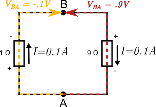
This result sounds very non-intuitive but it all comes down to the fact that the electric field is non-conservative in the presence of a changing magnetic field, therefor the voltage between any two points is not uniquely defined and depend on the path one takes between the points. This is quite easy to see in the figure below where the current is going around in a clockwise direction. A positive charge moving from the point A up to point B through the right resistor moves against the electric field while a positive charge which moves from the same point A up through the left resistor to B moves with the electric field, hence the voltages must be of opposite polarity.

Different paths give different voltages

A detailed analysis is provided by Romer in his paper What do voltmeters measure? . Walter Lewin also discusses this problem in more depth in the following video Kirchhoff’s Loop Rule Is For The Birds.

The claim by Walter Lewin that KVL doesn’t hold in this situation and that you must use Faraday’s law instead has generated some controversy, see for instance Does Kirchhoff’s Law Hold? Disagreeing with a Master by Mehdi Sadaghdar and the followup video by Lewin To Agree or Not to Agree with the Master that is Not what Matters.